01 What is an inverted pendulum?
An inverted pendulum is a pendulum in which its centre of mass is above the pivot point, making it unstable and prone to toppling without active control systems.
It can be controlled by moving the base. A basic example of this is balancing a ruler or a pencil on the tip of your finger by moving your finger so that the pencil’s centre of mass stays above the pivot. The schematic at the top of the page (Figure 1) displays the forces acting on the pendulum: gravity \(mg\) pulling the mass down, an external disturbance, ground friction, and the control force \(F\) applied through the base.
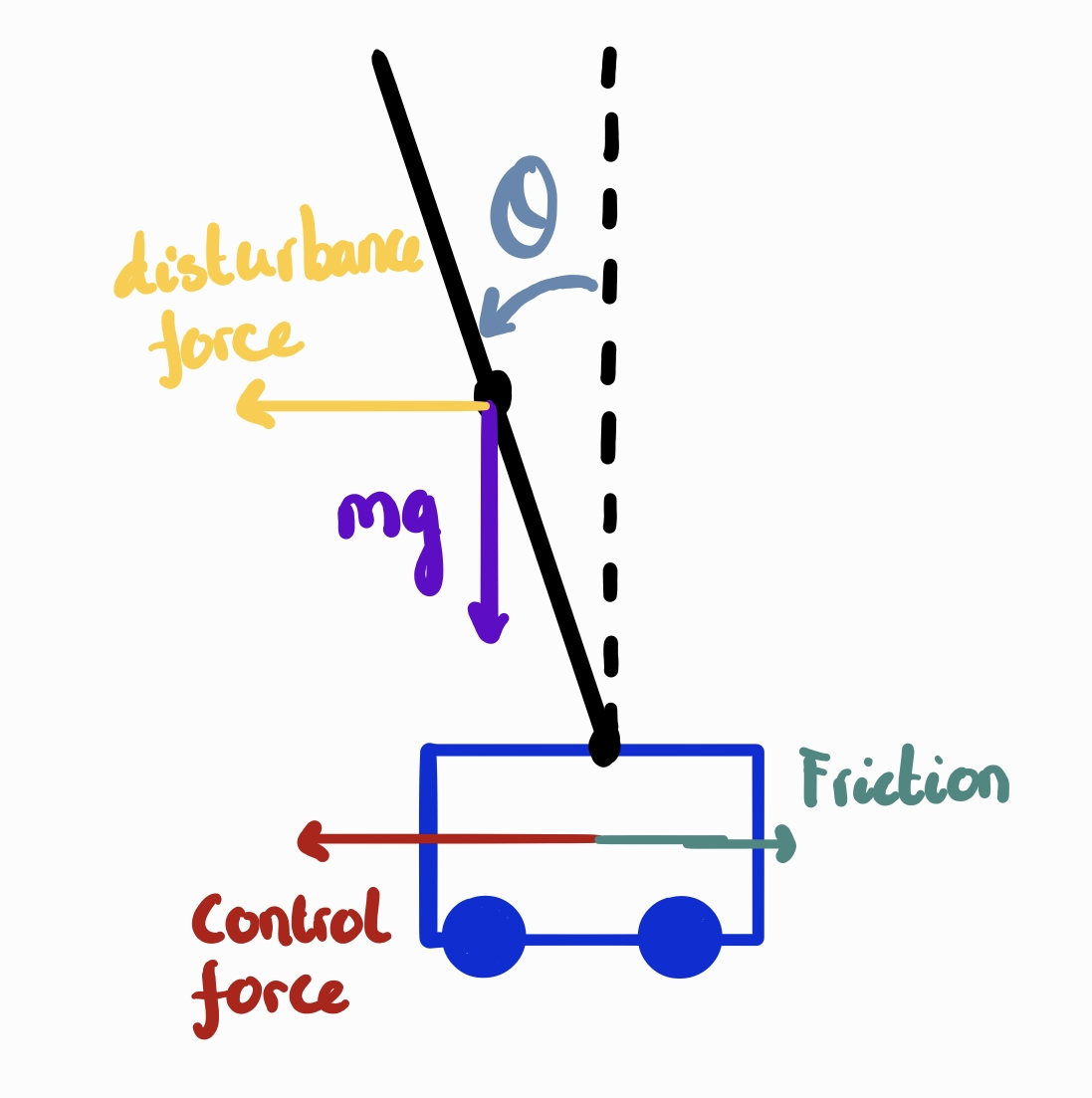
My original diagram of the inverted pendulum and the forces acting on it — recreated as the live schematic at the top of the page.
› Measurements
The diagram shown above (Figure 1) displays the forces acting on the pendulum. To control the pendulum, we need a way to calculate the force and acceleration required to move the base, given the angle, angular velocity, and mass, to ensure that the centre of mass is always above the base. To get these measurements in robotics, you need to use an IMU, which contains:
02 PID control (Proportional–Integral–Derivative)
The error term is the difference between the pendulum being perfectly upright when it is directly above the pivot point \(0\) rads and the pendulum’s actual angle at that moment.
P Proportional
The first part of PID control is the proportional term, known as the P value, and its equation is shown above. This applies a correcting force based on how far the pendulum is leaning away from the centre position (the error). A larger angle produces a greater corrective force, while a smaller angle produces a smaller one. Although this helps the pendulum respond quickly, proportional control alone can make the system unstable. This is because the pendulum may swing past the centre point at too high a speed, causing repeated side-to-side oscillations and making the robot unstable.
I Integral
The next part is the integral term, or I value, shown with the equation above. In some situations, proportional control may not produce sufficient force to fully balance the pendulum when the angle error is very small. Small continuous forces, such as gravity or friction, can still cause the pendulum to drift away from the centre over time. To fix this, the integral term tracks the total error over a period of time and adds a small extra correction to remove any remaining offset. However, the integral effect is normally kept quite low, because if too much past error is accumulated the system can become unstable and the pendulum movement may become even more erratic.
D Derivative
To help control this erratic movement, the derivative term is added and it is the equation shown above. The D value looks at the rate of change of the error rather than just the size of the error itself, acting as a braking force to slow the pendulum as it approaches the upright position. When the pendulum is moving rapidly towards the target angle, the derivative term produces an opposing effect that reduces the speed of the correction, as the rate of the error will be decreasing, creating a negative value. This makes the overall movement smoother and reduces overshoot and excessive oscillation.
Combining all these terms gives us the following equation, which can be used to control an inverted pendulum smoothly. (\(u(t)\) in a two-wheeled robot would be the motor voltage.)
Fig.02 — the setpoint and the measured angle meet at the summing junction; the error drives the PID controller, whose output moves the plant; the IMU and Kalman filter close the loop.
03 Potential issues with PID
› Windup
One potential problem with using PID control is an integral windup. This is because in a real-world scenario, motors have a physical limit where they can reach a maximum RPM, and if the system experiences a constant error, such as the pendulum being knocked over, this error will build up through the integral, causing it to request a higher RPM than is physically possible by the motor. However, the main issue is that when the robot returns to its correct position, the controller has to unwind all the accumulated excess error, causing the pendulum to overshoot significantly and fall over.
To fix this, an anti-windup method is used, with the most popular being clamping. Clamping is where it conditionally turns off the integrator by setting its error input to zero when two things happen: the controller outputs its saturation limit, and the error is trying to push the controller even further into that saturation limit. The integral is then turned back on when the error sign changes from + to − or − to +.
› Noise
Another huge issue is noise, which can be caused by motor vibration, sensor inaccuracies, external factors, etc. One of the biggest issues is high-frequency noise, as even when the amplitude is low, it can create a very high derivative value in the PID control, causing inaccuracies. This can be fixed through a filter.
One of the best filters you can use is the extended Kalman filter. A Kalman filter removes noise by continuously comparing a mathematical prediction of a system’s state, such as the precise tilt angle, against the actual, jittery sensor measurements it receives. It mathematically blends these two values using a dynamic weight called the Kalman gain, trusting whichever source currently has less uncertainty to calculate a smooth, accurate estimate of the true state.
04 LQR control system
An LQR system, compared to a PID control system, is a lot more complex. Developed 38 years after PID, in the 1960s, an LQR system model offers much better performance in terms of stability and control. However, it requires more computation and, in robots — unlike PID — requires encoders on the motors.
The rest of this paper is the maths behind LQR: the state vector, the equation \(\dot{X} = AX + Bu\), deriving the A and B matrices, full-state feedback, why a naive approach falls short, the Riccati equation, and finally a fully worked example with real numbers.
05 The state vector
To begin with, you have a state vector \(X\), and for a self-balancing robot it would be represented with 4 variables — a \(4\times1\) vector:
The state vector is useful because it encapsulates the system’s exact physical state, allowing the Linear Quadratic Regulator (LQR) to compute the single, mathematically optimal motor torque required to keep the robot upright. These are the definitions for the terms shown:
› Eigenvalues: how the robot knows if it is stable
In terms of how the robot knows if it is stabilised or falling, it uses eigenvalues — a scalar value, \(\lambda\). It is used to see if a robot is stabilised due to this equation:
This is important because the rate of change of \(x\) with respect to time equals \(\lambda x\), which says that the rate at which \(x\) changes is proportional to \(x\). This is an exponential function and can be represented as:
This shows that if \(\lambda > 0\) the robot will be unstable, as \(e^{\lambda t}\) will increase exponentially as time passes. If \(\lambda = 0\) or \(\lambda < 0\), it will be stable or stabilising respectively, as it would be decreasing to 0. The matrix \(A\) will have 4 distinct eigenvectors \((v_1,v_2,v_3,v_4)\) and also 4 distinct eigenvalues \((\lambda_1,\lambda_2,\lambda_3,\lambda_4)\). And to show the robot’s stability, we can sum each mode:
where \(C\) is the coefficient of the term when \(t = 0\).
Fig.03 — both start from the same small tilt. A stable controller forces every eigenvalue into the “settles” regime.
Putting everything together: \(\dot{X} = AX + Bu\).
So, to put the equation into words: the rate of change = the physics of the robot alone \((AX)\) + what you are commanding the robot to do \((Bu)\).
06 Deriving A and B
The first row of the matrix \(A\) takes out the robot’s rate of change of position \((\dot{x})\) from the state vector. As the first term in the \(\dot{X}\) vector in the equation \(\dot{X} = AX + Bu\) is \(\dot{x}\), we simply take \(\dot{x}\) from the state vector \(X\):
Row 3 will just be \(\begin{bmatrix} 0 & 0 & 0 & 1 \end{bmatrix}\), as we need \(\dot{\theta}\) from the state vector, which is just its 4th variable, since the 3rd variable in the \(\dot{X}\) vector is \(\dot{\theta}\).
For row 2, we are looking to obtain \(\ddot{x}\) in terms of \(\theta\) (the angle deviation from the perfect vertical position). And for row 4, we are looking to get \(\ddot{\theta}\) from \(\theta\). In order to find these, we begin applying Newton’s laws: one for the horizontal motion of the whole thing, one for the rotation of the body about its centre of mass. These are all the new terms in the following equations:
Equation (1) is total horizontal force = mass × acceleration for the system. Equation (2) is the rotational law for the body. The crucial term is \(-m\,g\,l\sin\theta\), which is gravity and is what topples the robot.
However, the problem with these equations is that they are not linear due to the \(\sin\theta\), \(\cos\theta\) and \(\dot{\theta}^{2}\) terms, and eigenvalues and \(AX + Bu\) are built for a linear system. To make the equations linear, we can use the small-angle approximation, since a balancing robot only needs to deal with small values of \(\theta\), and a good control system will keep \(\theta\) within a few degrees:
Fig.04 — inside the shaded band the straight line and the sine curve are indistinguishable, so the linear model is faithful while the robot stays near upright.
Now, by substituting the small-angle approximations into equations (1) and (2), we get these 2 linear equations:
Now we need to remove the two unknowns with one equation — that is, \(\ddot{x} = \,\ldots\) without having another \(\ddot{x}\) or \(\ddot{\theta}\) inside the equation. To do this, we solve it simultaneously and get a common denominator \(p\), and get the following equations:
And the results are:
Therefore, for row 2 it will be \(\begin{bmatrix} 0 & 0 & \frac{m^{2}gl^{2}}{p} & 0 \end{bmatrix}\), and for row 4 it will be \(\begin{bmatrix} 0 & 0 & \frac{mgl(M+m)}{p} & 0 \end{bmatrix}\), giving the final matrix:
For vector \(B\), the first row is 0, as we already get the \(\dot{x}\) value from the \(AX\) part of the equation. Row 3 is also 0, as once again we get \(\dot{\theta}\) from the \(AX\) part in \(\dot{X} = AX + Bu\). And for rows 2 and 4, we can use the values on the right-hand side of equations (5) and (6) (\(F\) can be interchanged with \(u\)).
› Showing that the system with matrix A will be unstable
By looking at just the angle and switching the motor off, so therefore \(F = 0\), we get the equation:
Unstable: \(\ddot{\theta} = \omega^{2}\theta\). Stable: \(\ddot{\theta} = -\omega^{2}\theta\). It is unstable because, when the growth-rate coefficient is positive, it leads to exponential growth. So the angle doesn’t swing back and forth; it just blows up instantly until the robot hits the floor.
07 Feedback control
We know that the control system is naturally unstable, and we now need to make it stable through feedback, where it measures the state and feeds back to determine the control input.
› Full-state feedback: u = −KX
One of the best ways to create a simple, powerful feedback rule is to make the control flow through a weighted combination of all the values in the state vector, and is shown as:
In addition, we use a negative \(K\) to counter the robot’s movement by pushing it in the opposite direction. The \(k\) values inside the \(K\) vector are referred to as gains. Now, by substituting \(u = -KX\) into the original equation, we get:
So, in order for the robot to be stable, the eigenvalues of \((A - BK)\) need to be negative, using the same logic shown in the \(\dot{X} = AX + Bu\) section, so the control system needs to use the \(BK\) value to steer the eigenvalues to be negative.
› Is the robot controllable?
To see if the robot is controllable, we use the controllability matrix, which is the following:
Here, \(B\) is the direction your input pushes immediately, \(AB\) is where the push is a moment later, then \(A^{2}B\) is a moment after that, and so on. Then, using MATLAB, we can calculate the rank, which shows how many dimensions of the state equation can be controlled. So if the rank is equal to 4, the system is controllable, and if it is less than 4, it is not controllable. We will assume our robot is controllable.
08 Why this isn’t the end
Firstly, an aggressive controller commands forces larger than the motor can output. As soon as the motor reaches its saturation limit, the linear design — which assumes the motor can output unlimited force — no longer describes what the LQR system wants.
In addition to this, the gains can be calculated through pole placement, where you first decide what you want your 4 eigenvalues to be (all negative, to ensure the robot is stable) and write them as a polynomial’s solutions:
and through this you get a quartic. Then you take the quartic from the equation \(\det(A - BK - \lambda I) = 0\), whose coefficients contain the unknown gains \(k_{1},k_{2},k_{3},k_{4}\), and you set the coefficients to equal each other, creating four different equations with four unknowns. By solving them simultaneously, you can find the \(k\) values.
When you set the two quartics to equal each other, you see that multiple \(k_{1},k_{2},k_{3},k_{4}\) values sit in one coefficient, so changing only one of the four gains shifts the other coefficients, which shifts all four eigenvalues at once. Therefore the four gains cannot be treated as 4 independent dials — there is no single gain that will control a single eigenvalue, and so you cannot tune the controller by changing one gain and watching just one eigenvalue respond.
The pole-placement method does not tell you where the four eigenvalues should be placed to make the robot behave well, as many different sets of negative eigenvalues all keep the robot stable. The behaviours you actually care about — how quickly the angle settles, how far the robot drifts along the floor, and how sensitive it is to sensor noise — don’t correspond neatly to individual eigenvalues either.
So designing a good controller this way becomes a process of trial and error: you guess a set of target eigenvalues, solve for the \(k\) values, simulate the result, and adjust. This gives no principled way of knowing whether the gains you finally settle on are the best ones possible, and also makes the process very time-intensive.
09 The Linear Quadratic Regulator
To fix the issues, we need to find another way to compute which stabilising gain \(k_{1},k_{2},k_{3},k_{4}\) is the best out of all the stabilising gains.
1 Scoring a controller with a cost function
So here we essentially try to compute a value that tells us how good the controller is — basically saying how good the \(k\) values are — where the lower the number, the better it is. There are two things that negatively impact the run:
- The state being away from zero, as we want \(\theta\) and \(x\) to be as close to zero as possible — we want it to be upright, still, and in place.
- Using a lot of control effort, because large motor forces drain the robot’s battery, can cause overheating, and the motors sometimes hit their physical limit, leading to harsh movements.
In order to create this scoring system, we need to be able to turn a vector into a single number value, and to do this we use the quadratic form. Given a vector \(X\) and a square matrix \(Q\), by calculating \(Qx\) and then \(x^{\mathsf{T}}(Qx)\) we get the following, which gives us a single value:
as a \(1 \times n\) row times an \(n \times n\) matrix times an \(n \times 1\) column gives a \(1 \times 1\) result. Now we can look at the LQR cost function, which is the following:
where the \(x^{\mathsf{T}}Qx\) is the state deviation and \(u^{\mathsf{T}}Ru\) is the control effort. Also, integration is used to sum up how bad the controller is over time. If the robot leans and moves for a long time, it will add up the badness from \(t=0\) to the infinite future.
2 What are Q and R?
We chose the matrices \(Q\) and \(R\), which are the only factors within the LQR control system that we choose, and everything else is done automatically.
- For \(Q\), each diagonal entry \(q_{1},q_{2},q_{3},q_{4}\) is how much we care about each state being zero. For example, setting \(q_{3}\) as a large number means that you prioritise the tilt angle being zero and hate any tilt.
- For \(R\), it is how much you care about saving control effort; the higher you set the value of \(R\), the more you are going easier on the robot’s motors.
- Overall, only the ratio matters, as it is the balance between \(Q\) and \(R\) and is what determines how the control system works. A large \((Q/R)\) ratio means the control system will be fast, aggressive and effortful; a small \((Q/R)\) ratio means it will be gentle and slow.
3 The answer
Now, by minimising \(J\), we use the following equation to find what the optimal value of \(K\) is:
where the matrix \(P\) is the (symmetric, positive semi-definite) solution of the Continuous Algebraic Riccati Equation (CARE):
where all of \(A,B,R,Q\) are known, and you use the equation to solve for \(P\). There is a long derivation for this formula, and also a way to solve for \(P\); however, in our case:
import numpy as np
from scipy.linalg import solve_continuous_are

P = solve_continuous_are(A, B, Q, R)10 How it works
Overall, to show how it works, I will lay out the processes the robot goes through for the LQR system.
Choose the physical parameters
The physical parameters are chosen, for example:
| Quantity | Symbol | Value |
|---|---|---|
| Wheel & base mass | \(M\) | \(0.5\ \text{kg}\) |
| Body mass | \(m\) | \(0.5\ \text{kg}\) |
| Height of body centre of mass above the axle | \(l\) | \(0.15\ \text{m}\) |
| Body moment of inertia \(=\tfrac{1}{3}ml^{2}\) | \(I\) | \(0.00375\ \mathrm{kg\,m^2}\) |
| Gravity | \(g\) | \(9.81\ \mathrm{m/s^2}\) |
And we also compute the value \(p\):
Compute the A and B matrices
Here we compute the A and B matrices:
So with these calculations, the A and B matrix is:
Check if it is unstable and controllable
In this step, we check if the robot is unstable and controllable, and to do this, we calculate the eigenvalues and use the controllability matrix. First, to check whether the robot is unstable, we compute the eigenvalues of \(A\) and ignore \(B\), since we are only looking at the robot’s state with no input. In order to find the eigenvalues of \(A\), we do \(\det(A - \lambda I) = 0\), which returns \(\lambda\) as:
The positive real part of the eigenvalue \(+8.86\) shows that the robot is naturally unstable. Then we use the controllability matrix \(\mathcal{C} = \begin{bmatrix} B & AB & A^{2}B & A^{3}B \end{bmatrix}\) and compute its rank, which returns a rank of 4, showing that the robot is able to steer all 4 states, so an LQR solution is guaranteed to exist.
Choose Q and R
Here we choose the values placed in the matrices \(Q\) and \(R\). For \(Q\), we care most about the tilt angle, as the robot falling is the main failure that we want to avoid, and we don’t care as much about the position and the rates. For \(R\), we set it to reflect that we are willing to expend a normal amount of motor effort.
So, essentially, we are saying we care 10 times more about the tilt angle than about all the other variables in the state vector.
Compute the optimal K values
Now compute the optimal \(K\) values. First, we use the Riccati solver to compute the matrix \(P\), and then \(K = R^{-1}B^{\mathsf{T}}P\) to return the \(K\) value, and in our case it will equal:
So, therefore, the motor command for each instant is:
And by looking at the values, we can see that \(k_{3}\) is by far the largest, as expected, indicating that a small deviation in the robot’s tilt angle will produce the largest corrective force. \(k_{4}\) reacts to how quickly the robot is tipping, catching a fall early rather than waiting for the tilt angle to increase; without it, the robot would overshoot and oscillate. Finally, \(k_{1}\) and \(k_{2}\) are smaller and gently keep the robot from drifting away while it balances.
Check whether it is actually stable
This is the final step, where we check whether the robot is actually stable by computing the eigenvalues of \(A - BK\), which return:
Since all the real parts of the eigenvalues are negative, the system is stable. This is because the real part of the eigenvalue represents the decay of the \(e^{\lambda t}\) term, and the imaginary part represents the oscillations. For example, looking at the eigenvalue \(-0.84 \pm 0.50\,i\): the real part is negative, so it will decay, but its magnitude is small, so it will decay slowly at around \(1/0.84 \approx 1.2\ \text{s}\); and the imaginary part means it oscillates at \(0.5\ \text{rad/s}\). Crucially, the decay time is much shorter than one oscillation period, so the motion dies away before the robot can complete one full swing, showing that it is well-damped: you will get roughly a single small overshoot which is then gone, rather than a sustained wobble.
Overall, putting the four eigenvalues together, the two fast eigenvalues \((-13.6\) and \(-6.1)\) snap the angle back quickly and handle most of the initial error, while the slow complex pair \((-0.84 \pm 0.50\,i)\) is what is left over and produces a gentle overshoot, followed by the slow final approach to rest.
Fig.05 — the lone unstable pole at \(+8.86\) is the problem; choosing \(K\) relocates the closed-loop eigenvalues to \(-13.63,\,-6.07,\,-0.84\pm0.50i\), all safely in the stable half-plane.
11 Putting it into a robot
While the maths will compute \(K\) for us, the robot still needs to measure its 4 states many times per second, compute \(u = -Kx\), and convert it into a motor command. A balancing robot runs the same short loop, typically 100–500 times every second, forever:
Fig.06 — and the \(u\) value is the force. Then we convert the force into PWM, allowing us to control the motors and stabilise it.
That tight loop is what turns a page of linear algebra into a robot that refuses to fall over — which is the project this paper was written alongside.
See it in hardware Self-Balancing Desk Robot Coming soon →